Uncertainty Principle

Chapter contents: Chapter 12: Quantum Mechanics

Probability Wave

The de Broglie wavelength assigns a wave nature to everything, even to the things we are used to thinking of as particles, such as an electron. So, what kind of waves are they? As far as we know, there are not smaller parts that electron can be broken into that can be oscillating. Furthermore, when we measure the position of the electron, each time, we find the electron at some definite location, as we would expect for a particle. So, what kind of a wave is electron?

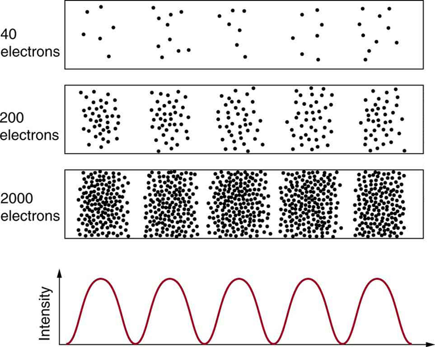
Figure 12.5.1 illustrates a result of electron interference experiment. Each dot represents the location where an electron was detected, and you see that with few electrons, dots appear spread out more or less randomly, and it is not obvious if there is any location where constructive interference or destructive interference is occurring. But as you continue to collect more data (more electrons detected), a pattern begins to emerge, where there are locations where electrons are mysteriously never detected. Those are the locations where electron waves—whatever they are—are destructively interfering.

A graph is shown for intensity which is varying like a wave. Corresponding to the maximum point of the wave electrons are shown as small dots in three strips. These strips show different number of electrons with varying density of dots along the length of the strip. A larger number of electrons are in the first strip, a smaller number of electrons in the second strip, and very few electrons in third strip. — **Figure 12.5.1.** The building up of the diffraction pattern of electrons scattered from a crystal surface. Each electron arrives at a definite location, which cannot be precisely predicted. The overall distribution shown at the bottom can be predicted as the diffraction of waves having the de Broglie wavelength of the electrons.

A double-slit interference wavelength pattern for electrons is shown in figure a and for photons in figure b. — **Figure 12.5.2.** Double-slit interference for electrons (a) and photons (b) is identical for equal wavelengths and equal slit separations. Both patterns are probability distributions in the sense that they are built up by individual particles traversing the apparatus, the paths of which are not individually predictable.

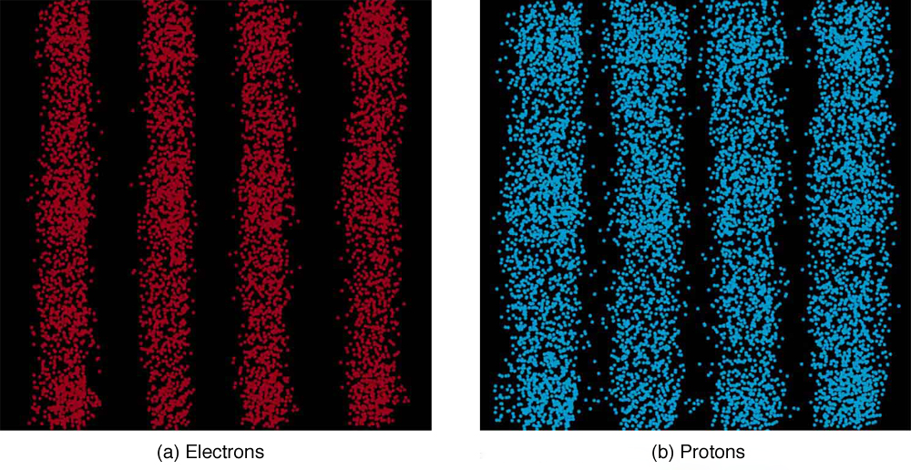
A wave function describes a quantum state and is used to calculate probabilities for measurement outcomes. For position measurements, the squared magnitude of the wave function gives a probability density. The phrase “probability wave” refers to this wave-like probability amplitude. The Schrödinger equation describes how the wave function evolves.

The most disquieting aspect of quantum mechanics is that the nature, at its most fundamental level, can only be described probabilistically. In Figure 12.5.1 and Figure 12.5.2 above, for each dot representing an electron or a photon, the experimental setup was identically. But with this identical set up, each electron (or each photon) ends up taking different paths, ending at the location represented by the dot. In classical mechanics, we would say this was because of our incomplete knowledge of the setup (we don’t know the precise way an electron bounces off from the barriers on its way to the screen where it is detected). In quantum mechanics, even in theory—assuming the most complete knowledge theoretically possible—we can only describe probability of finding the electron at one location, and the theory does not allow for prediction of individual electron paths. This aspect disturbed many physicists working on quantum mechanics, including Albert Einstein, who exclaimed, incorrectly, “God does not play dice.”

Heisenberg Uncertainty Principle

If the theory does not allow prediction of individual electron path, could we simply measure the location of the electron as it travels toward the screen? When such experiment was done, the experimenters found more than what paths the electrons took to result in the interference pattern. They found that the interference pattern itself was gone, with the constructive and destructive interference fringes smeared out!

Obtaining information about a quantum system requires an interaction with it. A measurement that distinguishes the paths through the slits changes the state of the system, so the alternatives no longer produce the same interference pattern.

For example, scattering a photon from an electron can transfer momentum to the electron. The measurement therefore affects the electron’s subsequent motion. The uncertainty principle discussed below describes an intrinsic restriction on quantum states, beyond the effects of a particular measurement procedure.

A photograph of a young, smiling Werner Heisenberg. — **Figure 12.5.3.** Werner Heisenberg was one of the best of those physicists who developed early quantum mechanics. Not only did his work enable a description of nature on the very small scale, it also changed our view of the availability of knowledge. Although he is universally recognized for his brilliance and the importance of his work (he received the Nobel Prize in 1932, for example), the fact that Heisenberg remained in Germany during World War II and headed the German effort to build a nuclear bomb is sometimes held against him. (credit: Author Unknown, via Wikimedia Commons)

A quantum state generally does not assign one definite value to every measurable quantity. If we prepare many systems in the same state and measure position, the results have a distribution; measurements of momentum have another distribution. The spreads in position and momentum obey Heisenberg’s uncertainty principle. A state with a very narrow position distribution must have a broad momentum distribution. This restriction is a property of quantum states, not merely a consequence of imperfect instruments or a disturbance caused by measurement. As an illustrative estimate, consider a localized wave packet whose position spread is comparable to its typical wavelength:

Δ x \approx λ

(12.5.1)

Such a localized wave packet contains a range of wavelengths and therefore a range of momenta. In this example, its momentum spread is of the same order as the momentum associated with the typical wavelength. Using the de Broglie relation gives the estimate

Δ p \approx p

, where

p = h / λ

(12.5.2)

For this family of wave packets, decreasing the position spread increases the momentum spread. Multiplying the two estimates cancels the typical wavelength, giving

Δ x Δ p \approx h

(12.5.3)

This illustrative estimate gives a product of spreads of order Planck’s constant. The precise lower bound depends on defining the spreads as standard deviations.

With position and momentum spreads defined as standard deviations, quantum mechanics gives the precise lower bound

Δ x Δ p \geq \frac{h}{4 π}

(12.5.4)

This is the Heisenberg uncertainty principle. The product of the position and momentum spreads cannot be smaller than the bound shown above. Reducing one spread raises the minimum possible value of the other.

An electron localized within an atom has a spread of momenta. A more tightly localized state requires a larger momentum spread. Quantum mechanics therefore describes the electron with a quantum state and its measurement probabilities, rather than a definite planetary orbit.

Example 12.5.1

Heisenberg Uncertainty Principle in Position and Momentum for an Atom

(a) If an electron in an atom has a position spread of 0.0100 nm, what is the minimum spread in its velocity? (b) What kinetic-energy scale corresponds to that velocity spread, in eV?

Strategy

The uncertainty in position is the specified spread of the electron’s quantum state,

Δ x = 0 . 0100 nm

. Thus the smallest uncertainty in momentum

Δ p

can be calculated using

Δ x Δ p \geq h /4 π

. Once the uncertainty in momentum

Δ p

is found, the uncertainty in velocity can be found from

Δ p = m Δ v

Solution for (a)

Using the equals sign in the uncertainty principle to express the minimum uncertainty, we have

Δ x Δ p = \frac{h}{4π}

Solving for

Δ p

and substituting known values gives

\begin{aligned} Δ p & = \frac{h}{4 π Δ x} = \frac{6.63 \times 10^{−34} J·s}{4 π (1.00 \times 10^{−11} m)} \\ = 5.28 \times 10^{−24} kg·m/s \end{aligned}

Thus,

Δ p = 5 . 28 \times 10^{−24} kg \cdot m/s = m Δ v

Solving for

Δ v

and substituting the mass of an electron gives

\begin{aligned} Δ v & = \frac{Δ p}{m} = \frac{5.28 \times 10^{−24} kg·m/s}{9.11 \times 10^{−31} kg} \\ = 5.79 \times 10^{6} m/s \end{aligned}

Solution for (b)

Although large, this velocity is not highly relativistic, and so the electron’s kinetic energy is

\begin{aligned} {KE}_{e} & = \frac{1}{2} m v^{2} \\ = \frac{1}{2} (9.11 \times 10^{−31} kg) {(5.79 \times 10^{6} m/s)}^{2} \\ = (1.53 \times 10^{−17} J) (\frac{1 eV}{1.60 \times 10^{−19} J}) \\ = 95.5 eV \end{aligned}

Discussion

An atomic size is roughly 0.1 nm, so a position spread of 0.0100 nm describes an electron localized within a small part of an atom. The associated minimum velocity spread corresponds to a kinetic-energy scale of 95.5 eV. This is larger than many atomic transition energies, showing that such tight localization has substantial energetic consequences.

Why don’t we notice this restriction in everyday life? Planck’s constant is very small on everyday scales. The minimum position and momentum spreads allowed for a macroscopic object can both be negligible for practical measurements. Classical mechanics then provides an excellent approximation, as expected from the correspondence principle.

Finally, note that in the discussion of particles and waves, we have stated that individual measurements produce precise or particle-like results. A definite position is determined each time we observe an electron, for example (represented as dots). But repeated measurements produce a spread in values consistent with wave characteristics, illustrating the underlying probability density. The great theoretical physicist Richard Feynman (1918–1988) commented, “What there are, are particles.” When you observe enough of them, they distribute themselves as you would expect for a wave phenomenon. However, what there are as they travel we cannot tell because, when we do try to measure, we affect the traveling.

Chapter section summaries

Continue to this item in the chapter review.Continue to this item in the chapter review.Continue to this item in the chapter review.Continue to this item in the chapter review.Continue to this item in the chapter review.Continue to this item in the chapter review.Continue to this item in the chapter review.

Chapter questions and exercises

Continue to this item in the chapter review.Continue to this item in the chapter review.Continue to this item in the chapter review.Continue to this item in the chapter review.

Chapter glossary